Written by James Bowden, with thanks to Jenn and Sergey, Cat Glossop, Aileen Zhang, and Shreshth Srivastava for feedback.
Choose your own adventure (pick the one best suited to your expertise):
In the era of AI-driven science and engineering, we often want to design proteins, materials, circuits, etc. in silico according to user-specified properties (e.g., that a protein binds its target; above: top left). Given a property predictive model, \(f(x)\), in silico design typically involves training a generative model over the design space to concentrate on designs with the desired properties (above: bottom left). This is in general challenging due to the combinatorial nature of the design space. However, many property predictors in scientific applications are decomposable—for example, the amino acids contacting a binding target may need to only loosely interact with the rest of the protein (above: top right). In cases where this decomposability is sufficiently simple (e.g., fully separate components), it can be straightforward to account for manually, but in the general case of arbitrarily complex decompositions, as represented by an interaction graph on design variables, a more systematic approach is needed. We present our method, DADO, which leverages decomposability to identify promising designs more quickly (above: bottom right), and discuss how one might obtain an appropriate decomposition in practice.
Design in discrete spaces, such as searching for the sequence of a protein that will bind a target (above: top left), is made difficult by the combinatorially large space that must be searched (above: bottom left). We argue that scientific design problems often exhibit some level of decomposability (above: top right) and explain how harnessing this can massively shrink the effective design space, allowing one to find desirable designs more efficiently. To take advantage of this smaller, decomposed design space, we present DADO, a method that infuses the standard distributional optimization algorithm with awareness of the decomposition such that it operates in the decomposed design space (above: bottom right), and uses message-passing to coordinate optimization across the search distribution factors. DADO operates on any decomposition, as represented by an interaction graph over design variables.
RL typically assumes access to a reward function which decomposes in a linear additive manner across timesteps in an MDP—allowing for efficient policy optimization via dynamic programming. In the typical scientific design setting, our task is to train a distribution over an object, such as a protein sequence, whose variables interact in complex, nonlinear ways to influence the reward function. As such, rather than maximizing a time-decomposed reward (i.e., a chain interaction graph), we generalize policy optimization to reward functions with arbitrary interaction graphs. After converting an input interaction graph into a junction tree, our method, DADO, factorizes its policy (or "search distribution") according to the junction tree and performs weighted regression with value functions estimated over the junction tree. Compared to a naive policy optimization algorithm (analogous to using a trajectory-level reward function; above: left), DADO's update is more statistically efficient and in practice, finds optimal designs more quickly (above: right).
This blog post will focus on protein design for concreteness. Optional details are collapsed (like \(m^{ath}\) or domain-specific particulars); without these, it should be a ~5 min read.
[optional]How can we formalize protein sequence design as an optimization problem? Though our method can be used for any optimization problem over a discrete design space, as a concrete example, let's consider only the problem of designing a protein sequence. We can set this up as follows:
The kind of discrete object that we'd like to design, \(x\), is a protein sequence of length \(L\) in which each design variable (or "position"), \(x_i\), is an amino acid from an alphabet, \(A_i\). For simplicity, we'll assume that every position uses the same standard amino acid alphabet of size 20, \(A\).
Given \(L\) and \(A\), we can write the design space as \(X := A^L\), i.e., all amino acid sequences of length \(L\). It follows that there are \(\lvert A\rvert^L=20^L\) possible proteins to choose from.
Specify a property function to design toward, \(f(x)\), such as binding affinity to a target, or gene editing efficiency. In practice, this may be a predictive model fit on limited assay-labeled data.
Putting this all together, our design problem is to find a sequence that maximizes our specification: \(x^{\ast}=\arg\max_{x\in X} f(x)\).
[optional]How are discrete optimization problems solved with standard distributional optimization? Distributional optimization is a way of solving design problems that can be written as \(x^{\ast}=\arg\max_{x\in X} f(x)\); estimation of distribution algorithms (EDAs) and policy optimization in reinforcement learning are two common instantiations. Compared to naively evaluating one protein, then the next, until all of \(X\) has been considered, distributional optimization algorithms navigate the design space using a probability distribution, \(p_\theta(x)\), often referred to as a "search distribution" or a "policy". Intuitively, the search distribution is like a spotlight that moves through the design space toward regions where \(f(x)\) is larger, by maximizing \(\mathbb{E}_{p_\theta(x)}[f(x)]\) (schematic: bottom left). In modern times, \(p_\theta(x)\) is typically parameterized as a highly expressive neural network generative model, like an autoregressive model or diffusion model, allowing for pretty arbitrarily shaped spotlights. Initializing \(p_\theta(x)\): \(p_\theta(x)\) might also be initialized as some pre-trained model, in which case we would in effect be implementing a kind of RL fine-tuning (with \(f\) as the reward signal). Alternatively, one might initialize \(p_\theta(x)\) to be a uniform distribution on a certain set of designs, e.g., those tested in an initial experiment, or initialize it completely at random. Standard EDA pseudocode
Sample from \(p_\theta(x)\) up to your experimental budget and test in the lab!
There's much more discussion of EDAs, their derivation, relevant hyperparameters, and the important ways they can be extended in our paper.
Decomposing the design space
A crux of many difficult design problems is that there are a huge number of possible designs—far too many to consider them all. However, we often have information that can help us decompose the design space and thereby search a much smaller area. For example, protein sequence design workflows assume, roughly, that the binding interface of a protein and the scaffold can be designed separately (sometimes called a scaffolding problem; schematic: top right). We call this a decomposition, and represent it with a graph in which nodes are design variables (amino acid positions) and edges denote coupling with respect to the property function. So, our example decomposition would be represented by a graph in which all interface amino acids are connected by edges, and all scaffold amino acids are connected by edges, but there are no edges between the interface and scaffold amino acids. We don't expect such clean-cut decomposability in most problems. Our core contribution is a design algorithm that can leverage any decomposability in the property function.
A crux of many difficult design problems is that there are a huge number of possible designs—far too many to consider them all. Imagine if, however, a (particularly simple) decomposition held—yielding two completely separate, smaller design spaces representing respectively the interface amino acids and the scaffold amino acids (schematic: top right). This decomposition corresponds to a linear additive form of the property function to be maximized, $f(x_i, x_s) = f_i(x_i) + f_s(x_s)$, from which we can see that this is actually two separate optimization problems: $$[x_i^{\ast}, x_s^{\ast}] = \arg\max_{x_i,x_s} f(x_i, x_s) = [\arg\max_{x_i} f_i(x_i), \arg\max_{x_s} f_s(x_s)]$$ If \(x_i\) has \(6\) design variables and \(x_s\) has \(9\) (as in the schematic), this yields a massive reduction in the size of the search space from \(20^{15}\) to \(20^6 + 20^9\). We don't expect such clean-cut decomposability in most problems. To allow more complex forms of decomposability, we represent a decomposition as a graph in which nodes are design variables and edges denote coupling with respect to $f(x)$; the simple example corresponds to two disconnected components. Our core contribution is a search algorithm that can leverage arbitrarily complex decomposition graphs.
Unlike in typical RL settings, for scientific design we can omit both time and the state-action distinction. There's no stochastic environment and the reward function is defined only on design variables, which you can think of as the actions. In RL, the decomposition graph would have as its nodes state-action pairs for each timestep, and edges only between subsequent timesteps, resulting in a chain. Ignoring this chain decomposition and performing policy optimization would amount to searching the space of all possible trajectories, which grows exponentially with the number of nodes in the graph (timesteps). By analogy, our decomposition graph has instead design variables for nodes (amino acid positions in the case of protein sequence design), and these variables can be coupled with respect to the reward function by arbitrarily complex graph topologies (i.e., not chains, or even trees). Our core contribution is a policy optimization algorithm that can leverage any decomposition graph topology.
What do realistic decompositions look like? Let’s look at decomposition graphs derived from two proteins, AAV and CreiLOV.
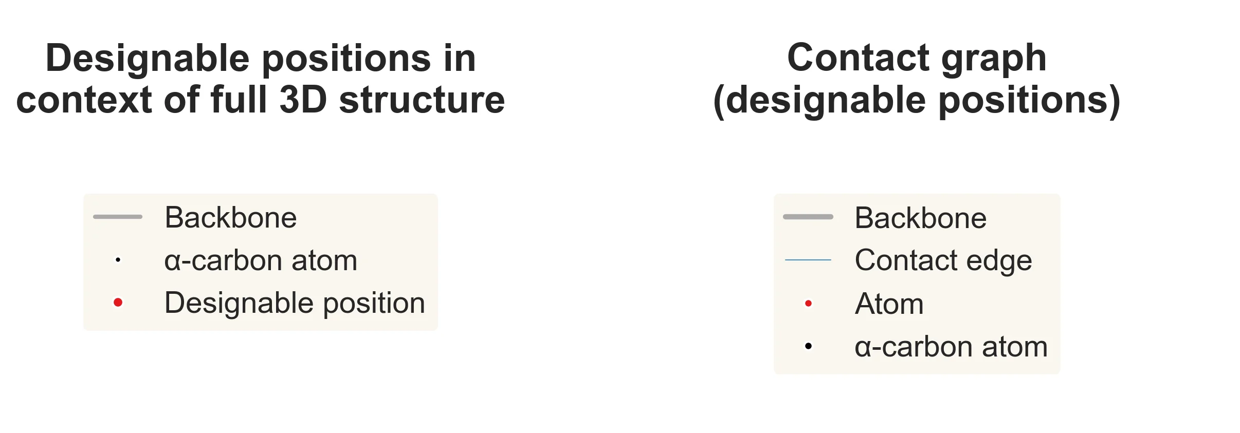
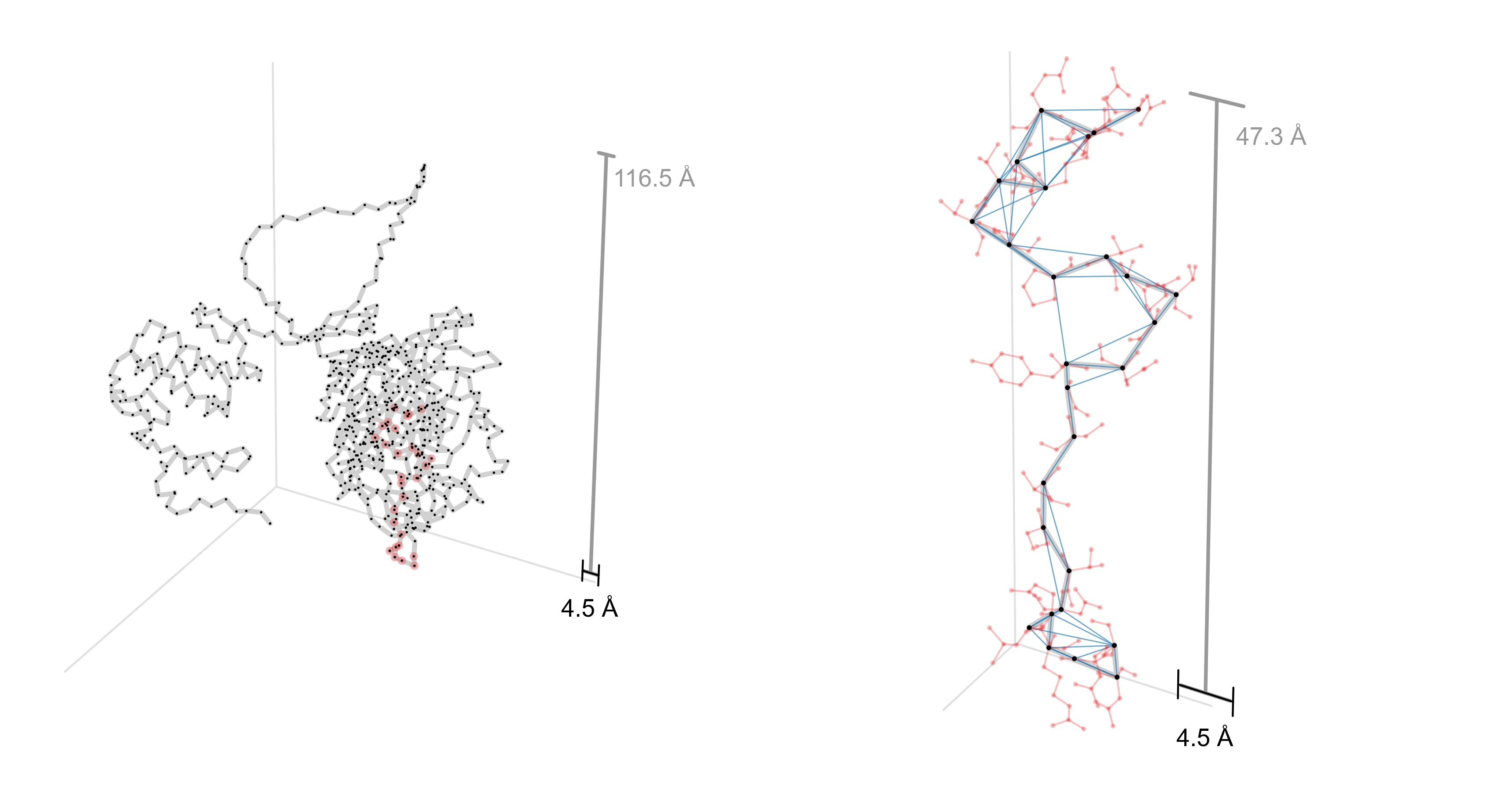
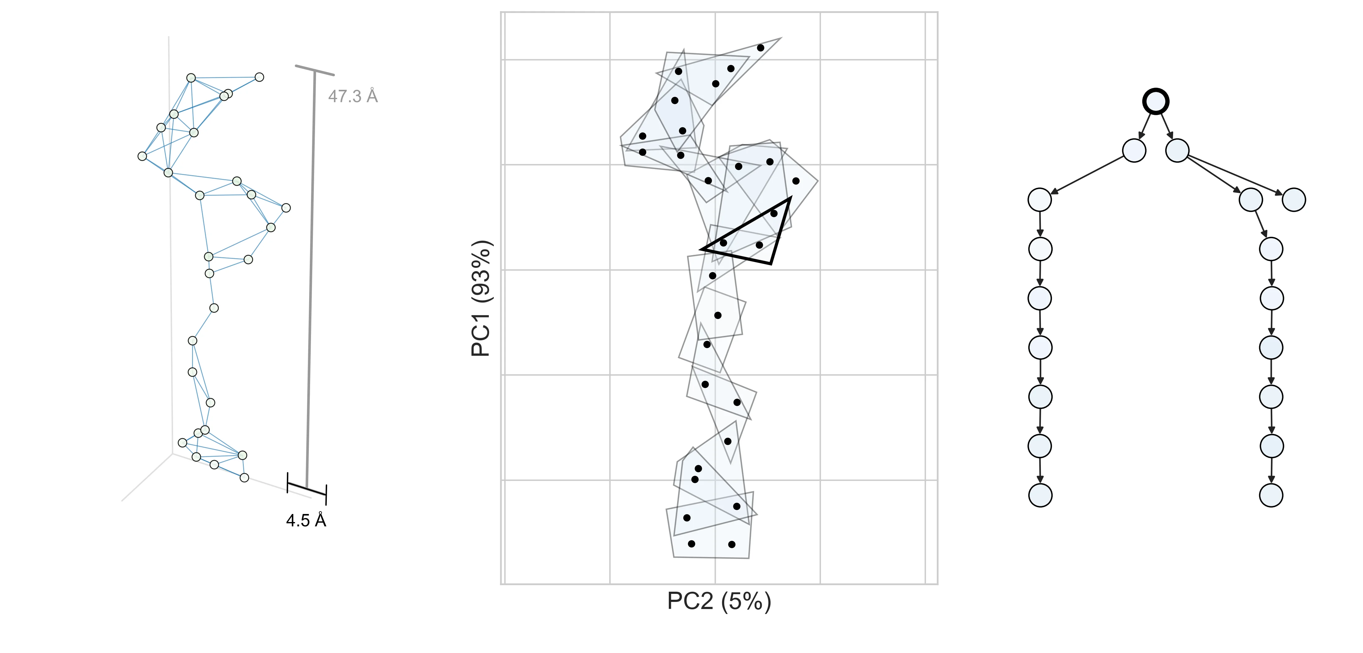
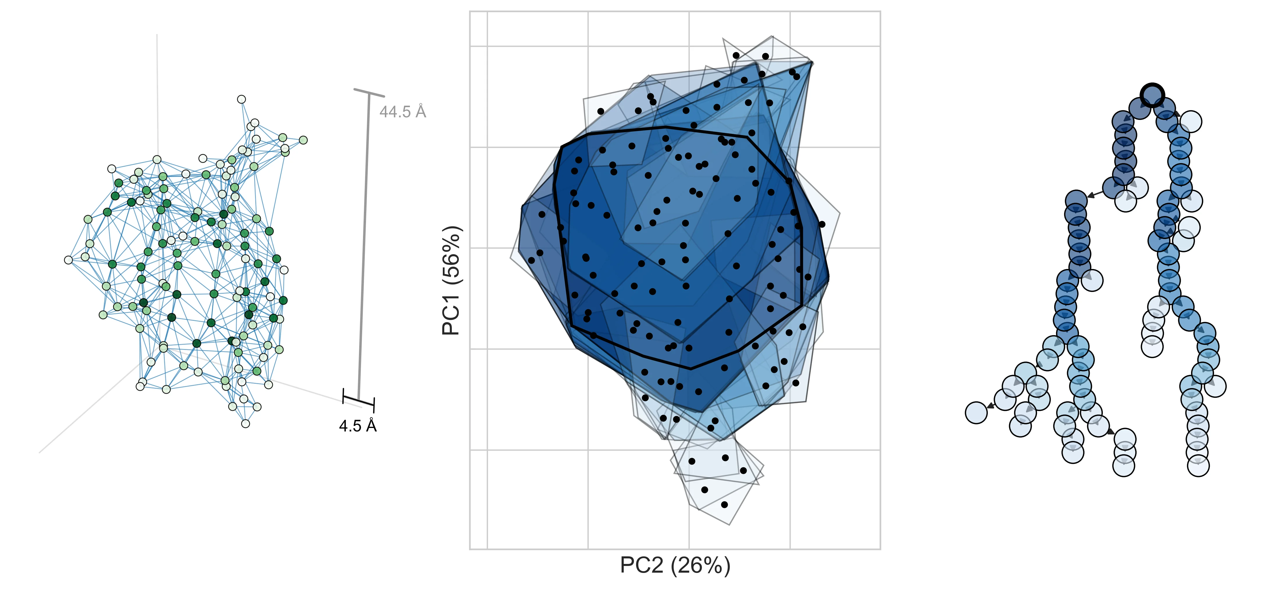
In the first figure, we show one way to obtain a decomposition graph for a protein design problem—by computing a contact graph. For two proteins, AAV VP1 (which co-assembles into a virus capsid) and CreiLOV (an oxygen-independent fluorophore), we first obtain a 3D structure from AlphaFold3 (left). To extract a decomposition graph from the 3D structure, we compute distances between all pairs of designable positions and create an edge if they’re within 4.5Å of each other (right).
a, AAV
b, CreiLOV
Notice that the decomposition graph for AAV (right) has few edges and is relatively chain-like. This suggests that we will be able to realize a large efficiency gain by operating in its decomposed design space. On the other hand, CreiLOV looks a lot more like a fully-connected graph. In this case, we can’t expect to improve over a naive optimization method which considers all variables jointly. One could always choose a more sparsely-connected decomposition (e.g., by lowering the contact distance threshold) such that it yields a larger potential efficiency gain. This hints at a key tradeoff in practice: the more decomposed the problem, the more efficiently it can be optimized, but if the chosen decomposition is too aggressive, it might preclude performant designs from being found.
Briefly, we can easily convert any undirected graph into a directed junction tree, which has no cycles, allowing DADO to draw inspiration from exact message-passing (next section). The corresponding junction tree for each protein is shown below (right), with additional visualizations to highlight its relation to the original decomposition graph (left, middle).
To infuse distributional optimization with knowledge of a decomposition graph, our method has two core components:
First, we perform search with a generative model, \(p_\theta(x)\), factorized according to the decomposition junction tree. Each factor distribution searches a subset of design variables corresponding to a node in the tree. This factorization makes it so that DADO only "sees" the smaller decomposed space1; whereas the standard EDA searches all dimensions of \(x\) together.
First, we perform search with a generative model, \(p_\theta(x)\), factorized according to the decomposition junction tree. Each factor distribution searches a subset of design variables corresponding to a node in the tree. This factorization makes it so that DADO only "sees" the smaller decomposed space1; whereas the standard EDA searches all dimensions of \(x\) together.
First, we perform search with a policy, \(p_\theta(x)\), factorized not in time but according to the decomposition junction tree. Each policy factor \(p_\theta(x_i \mid x_p)\) searches a subset of design variables corresponding to node \(i\) in the tree, conditioned on its parent node \(p\)'s variables.
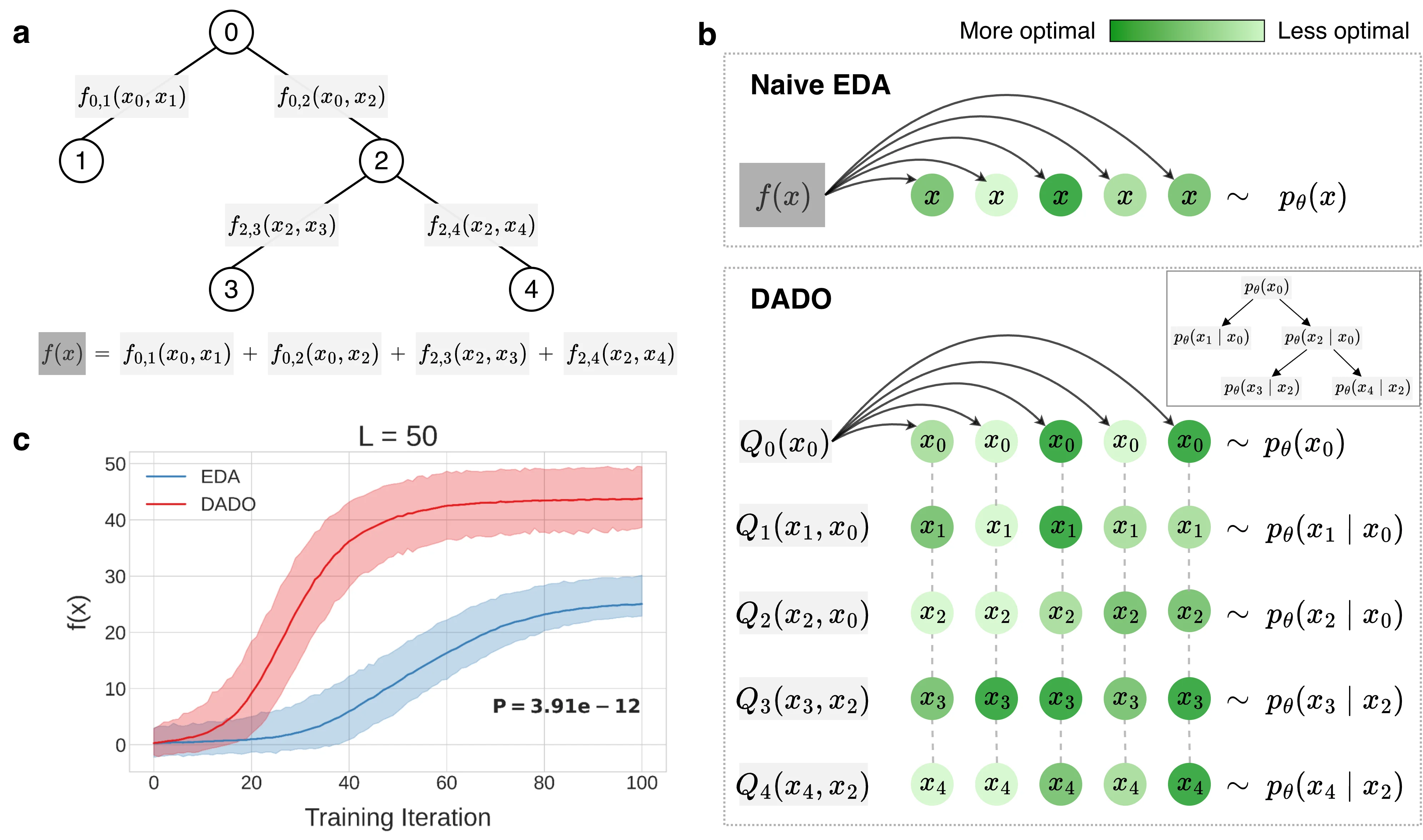
Second, we coordinate the generative model's factor distributions via message-passing. In essence, the messages (also called "value functions" and denoted \(Q_i(\tilde{x}_i, \tilde{x}_p)\)) describe how changing a single factor distribution affects its descendants in the tree, so that each factor can be updated in a manner that considers the design variables it has no direct control over. For more details, see the machine learning explanation (or the paper). The upshot is that this leads to a more statistically efficient optimization algorithm that navigates the space of designs more effectively. Below, we show a schematic comparison of a standard EDA to DADO (panel b) for a particular tree decomposition (panel a); on synthetic problems DADO consistently finds higher-\(f(x)\) designs (panel c).
Second, we coordinate the factor distributions via graph message-passing so that they can each be trained separately. The messages are called value functions and denoted \(Q_i(\tilde{x}_i, \tilde{x}_p)\); they are passed from the leaves of the junction tree to the root, communicating to each parent node the status of its children. Each \(Q_i(\tilde{x}_i, \tilde{x}_p)\) describes the partial value of \(f\) on the subtree rooted at node \(i\), in expectation over its descendants' search distributions. Each node aggregates all of its children’s value functions into its own and then uses it to shift its search distribution optimally with respect to its children. We can use the value functions to perform a weighted maximum likelihood update to each factor distribution separately, which makes DADO more statistically efficient than the standard EDA: each lower-dimensional distribution is updated using the full sample budget. Decentralized updates are possible because the value functions provide explicit coordination across all design variables (most importantly, those out of scope). The conditional dependence of each search distribution factor and value function closes the loop: each node responds to whichever partial designs are sampled from its parent’s search distribution. As a consequence, all coordination flows through the root node, which indirectly aggregates value functions from all other nodes in the junction tree and upon whose samples all other nodes are indirectly conditioned. Below, we show a schematic comparison of a standard EDA to DADO (panel b) for a particular tree decomposition (panel a); on synthetic problems DADO consistently finds higher-\(f(x)\) designs (panel c).
Second, we coordinate the policy factors with value functions, \(Q_i(\tilde{x}_i, \tilde{x}_p)\), which describe the partial value of \(f\) on the subtree rooted at node \(i\), in expectation over its descendants' policies. Each node aggregates all of its children’s value functions into its own and then uses it to shift its policy optimally with respect to its children. Then we perform an RWR/AWR-style weighed maximum likelihood update to each policy factor separately. This makes DADO more statistically efficient than the naive policy optimization algorithm (EDA), as each lower-dimensional distribution is updated using the full sample budget. Below, we show a schematic comparison of a standard EDA to DADO (panel b) for a particular tree decomposition (panel a); on synthetic problems DADO consistently finds higher-\(f(x)\) designs (panel c).
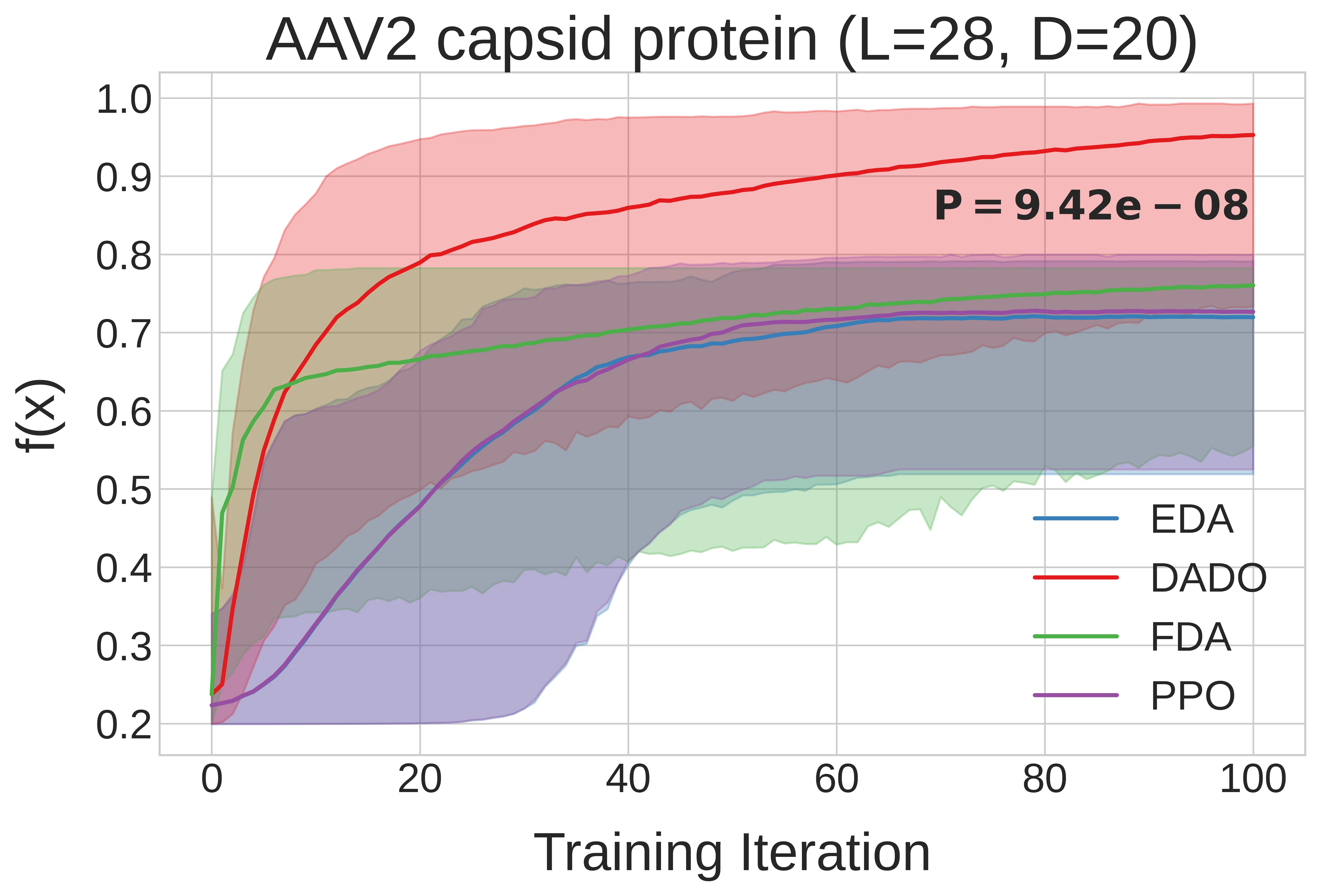
DADO’s optimization efficiency gain holds up for messier, real-world design problems too. Recall the two protein design problems we introduced earlier, AAV and CreiLOV, and their contrasting decomposition graphs (sparse vs. dense). Below2, we observe that DADO finds much better designs than decomposition-unaware methods for AAV design, whereas for CreiLOV, knowledge of the decomposition doesn’t help, as one would expect.
a
b
What now?
Finding an accurate decomposition for a design problem is not always straightforward. The real world is often structured though, and even very approximate decompositions can be useful. One might try to infer decomposability from labeled data or auxiliary information, or some other creative scheme. This is an exciting research direction both for proteins and scientific design in general.
For concreteness, here are some examples of scientific design problems with modularity that might lend itself to decomposition.
In natural systems, useful physical models often approximate interactions as primarily local, giving rise to sparse decompositions. In designing a crystal to minimize formation energy or maximize stability, for example, one might model atoms in a lattice as only directly interacting with their nearest neighbors. Or, consider the problem of designing a layered material for thermal or acoustic insulation. When choosing the material of each layer, we might assume that it mainly interacts with its direct neighbors—heat or sound has to pass through one layer to reach the next. As a result, one could optimize a thick stack of layers as decomposing according to a chain graph instead of a fully-connected one.
Modularity abounds in man-made systems. In the case of circuit design, usually not all components are directly connected by wires—so if trying to choose what type of component to put in each slot (assuming a pre-fixed topology) in order to minimize capacitance, one might model the system as sparsely-connected according to the wires. That is, that components only indirectly interact with other components if there is no direct wire between them. Similarly, in optical design of e.g., a research telescope, one might minimize wavefront error with respect to the physical parameters of a set of lenses/mirrors laid out in a pre-specified topology. For a given scene, interactions take place primarily via light passed between neighboring components, which in turn propagate a light field to the next components. One can imagine similar relationships between components of a mechanical system (e.g., a robot's limbs and actuators, with respect to torque costs or material stress).
There's no reason why DADO can't be used for optimization in continuous design spaces; we simply didn't investigate it in our paper. Everything should extend straightforwardly.
We hope you’ll read (and enjoy) our paper! If you’d like, you can return to the top and re-read from a different perspective :) Feel free to email me with any questions, comments or feedback. I’d also be excited to discuss applying our method to your problem, or potential collaboration.
Footnotes
In our paper, we include a baseline—a modernized version of the factorized distribution algorithm, or FDA—that only uses a factorization of the search distribution without the message-passing coordination. In FDA, the factorized search distribution is updated the same way as the standard EDA, with a per-sample weight, \(f(x)\), instead of a per-node weight. It's interesting that for a few problems, FDA performs as well as or better than DADO, despite its search distribution update being less statistically efficient. We suspect this is due to an additional source of variance—the sample-based approximation of DADO's value functions—which can outweigh the benefit of a per-node update. We only observed this when the junction tree nodes were relatively large, which is exactly when estimating a value function from finite samples is most difficult. It would be interesting to more carefully characterize this behavior, and one might adapt variance-reduction techniques from RL (like learned value functions) here. ↩
The y-axes between the two plots are not comparable; \(f(x)\) is protein-specific. For AAV, \(f\) represents viral viability (whether the capsid packages), and for CreiLOV, \(f\) represents fluorescence intensity. The upshot being that DADO can find better protein sequences than decomposition-unaware methods for AAV packaging, but cannot for CreiLOV fluorescence intensity. One should not conclude that the methods perform better on CreiLOV than on AAV or vice versa, as \(f\) is not comparable between them. ↩
 a, AAV
 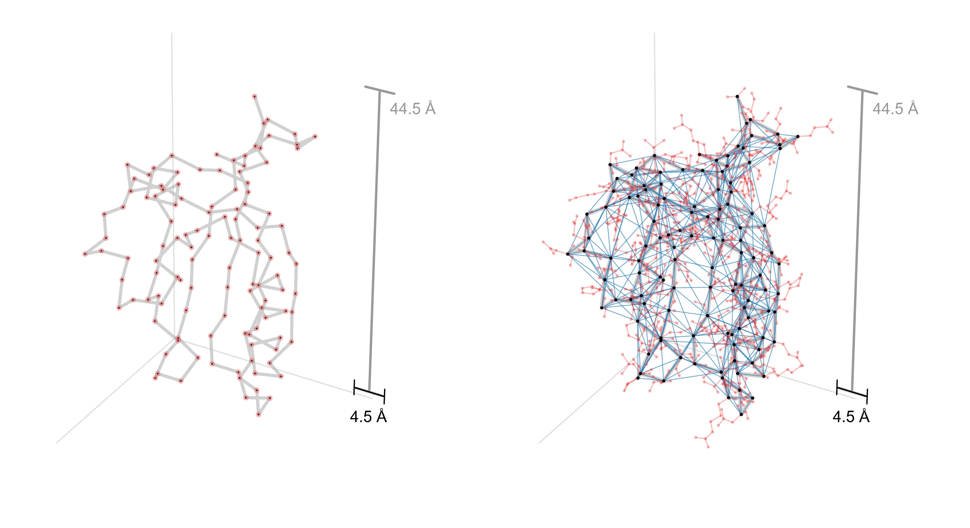 b, CreiLOV
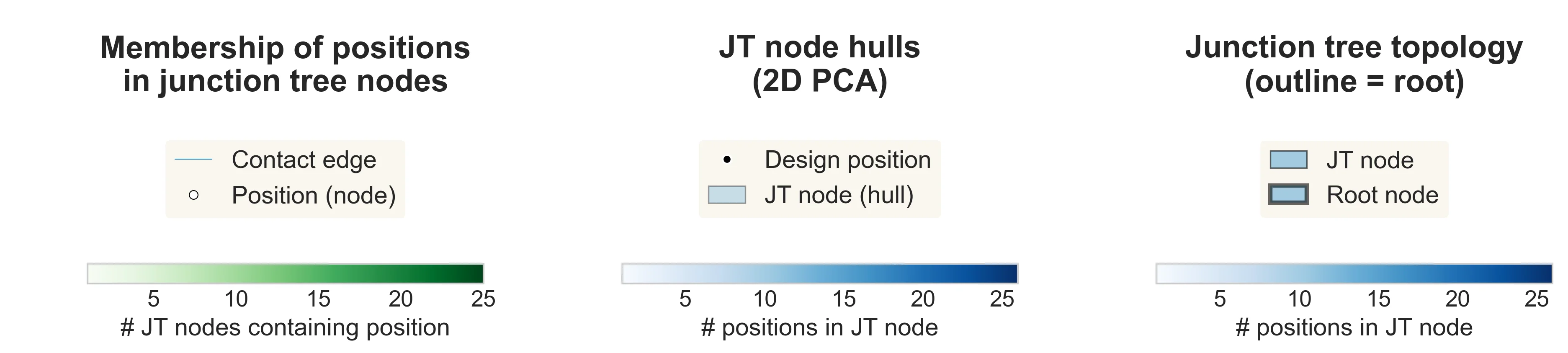
 a
a 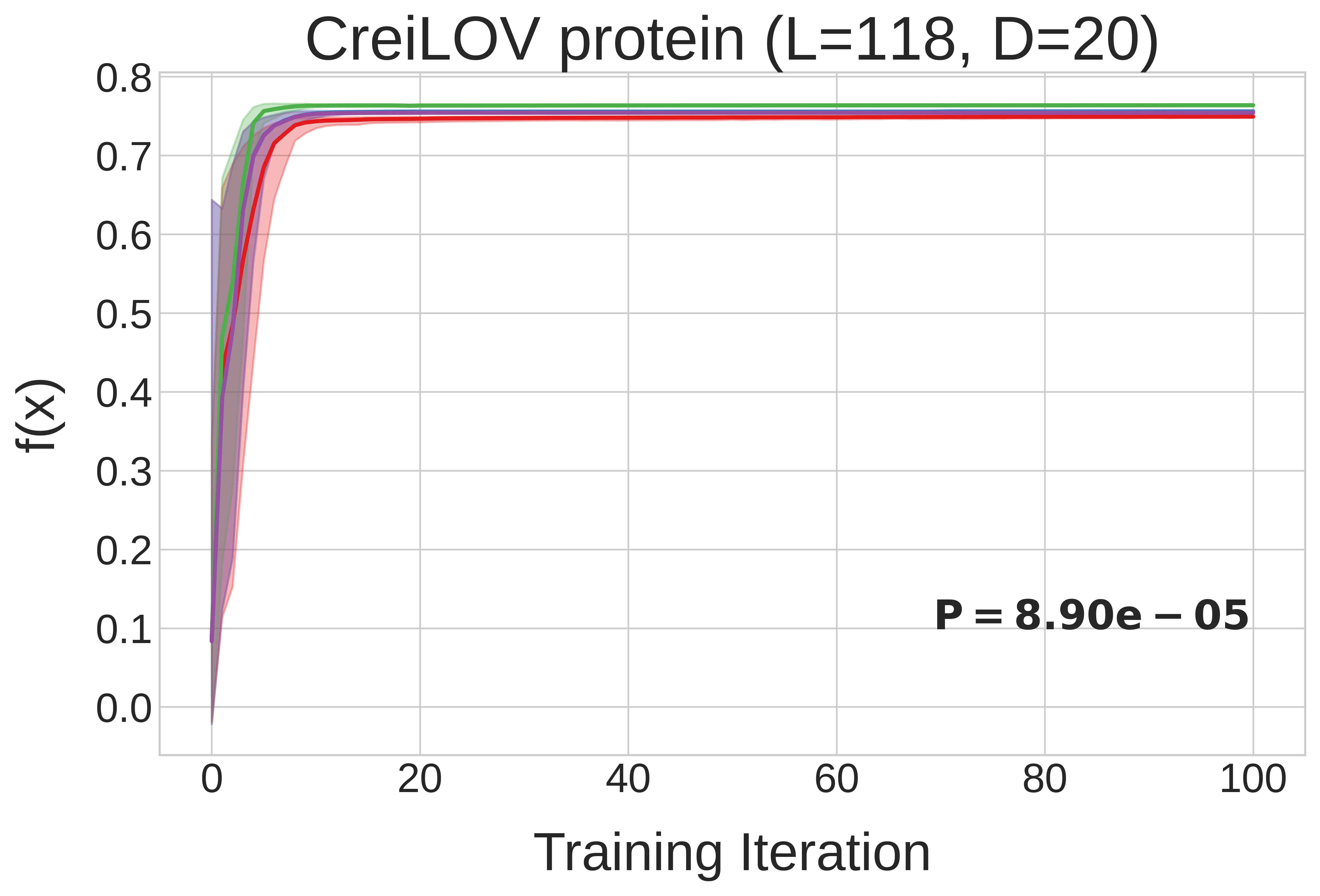 b
b