Gauge fixing for sequence-function relationships Anna Posfai, Juannan Zhou, David M. McCandlish, and Justin B. Kinney biorxiv, 2024

Gauges are a framework for fixing excess degrees of freedom so that your parameters can be interpreted more clearly (not so if multiple parameter values can yield same predictions, same model performance). ZSG and WTG are most commonly used but these can be generalized to hierarchical gauges which are defined by a regularization parameter (by order interaction) and a probability distribution on positions/identities. In fact, these two gauges correspond to hierarchical gauges with the uniform and delta (on WT sequence) distributions, respectively. Once a gauge has been fixed, interpretation can proceed. Other content that may be worth reading in the future, but stopping here for now. ^74edf6

Preliminaries (p 2-4)

Linear Models

Linear function of parameters \(\theta\). Sequences \(s\) may be embedded in some feature space \(x(s)\) which need not be linear.

One-hot models (OHE)

A type of feature embedding for sequences. Each AA @ each position gets a binary indicator. This means that a linear model on OHE feature space can be easily interpreted, as there’s a coefficient measuring contribution of a specific AA @ a specific position being present. OHE can also be used for pairwise or higher order modeling, where a higher-order term is 1 if all positions included in it take on the specified AAs, and is 0 otherwise.

Gauge freedoms

Def. transformations of model params \(\theta\) that leave all predictions unchanged. Generally, we can write \(g \in \mathbb{R}^{m} \text{s.t.} f(s; \theta) = f(s; \theta + g)\; \forall \; s \in \mathcal{S}\)¹.

For linear models

For a linear model, can write \(X \cdot g = 0\) for \(X \in \mathbb{R}^{N\times M}\) a feature matrix with rows corresponding to different sequences (datapoints).This implies that the columns of \(X\) (sequence features) aren’t linearly independent². Each linear relation btwn multiple columns specified by the model gives a gauge freedom \(g\). For an additive model over \(L\) positions, have \(L\) gauge freedoms because we know that \(x_{0(s)}= \sum\limits_{c}(x_l^c(s))\)³. Concretely, this means that for a given position, one could change \(\theta_0\) and this would correspond to a change in \(\theta_l\) that would leave all predictions the same as before. In other words, we can compensate for parameter changes, meaning there are excess degrees of freedom.

More general models

Pairwise models inherit the \(L\) DoFs from the additive model and additionally get \(\binom{L}{2}\cdot (2\alpha-1)\) gauge freedoms from linear relations between the pair terms and the single-position terms. The more general principle is that summing a \(K\)-order feature over the whole alphabet at a chosen position gives a feature of order \(K-1\) — effectively, you can marginalize (a la Stephan’s Selection Probabilistic Model; could try to think more clearly about connections).

Parameter values depend on choice of gauge

Cannot really interpret parameters if they can take on many different values with the same effect. Strategy: fix a gauge, meaning adopting constraints that will eliminate DoFs.

Example (figure) in 3 different gauges

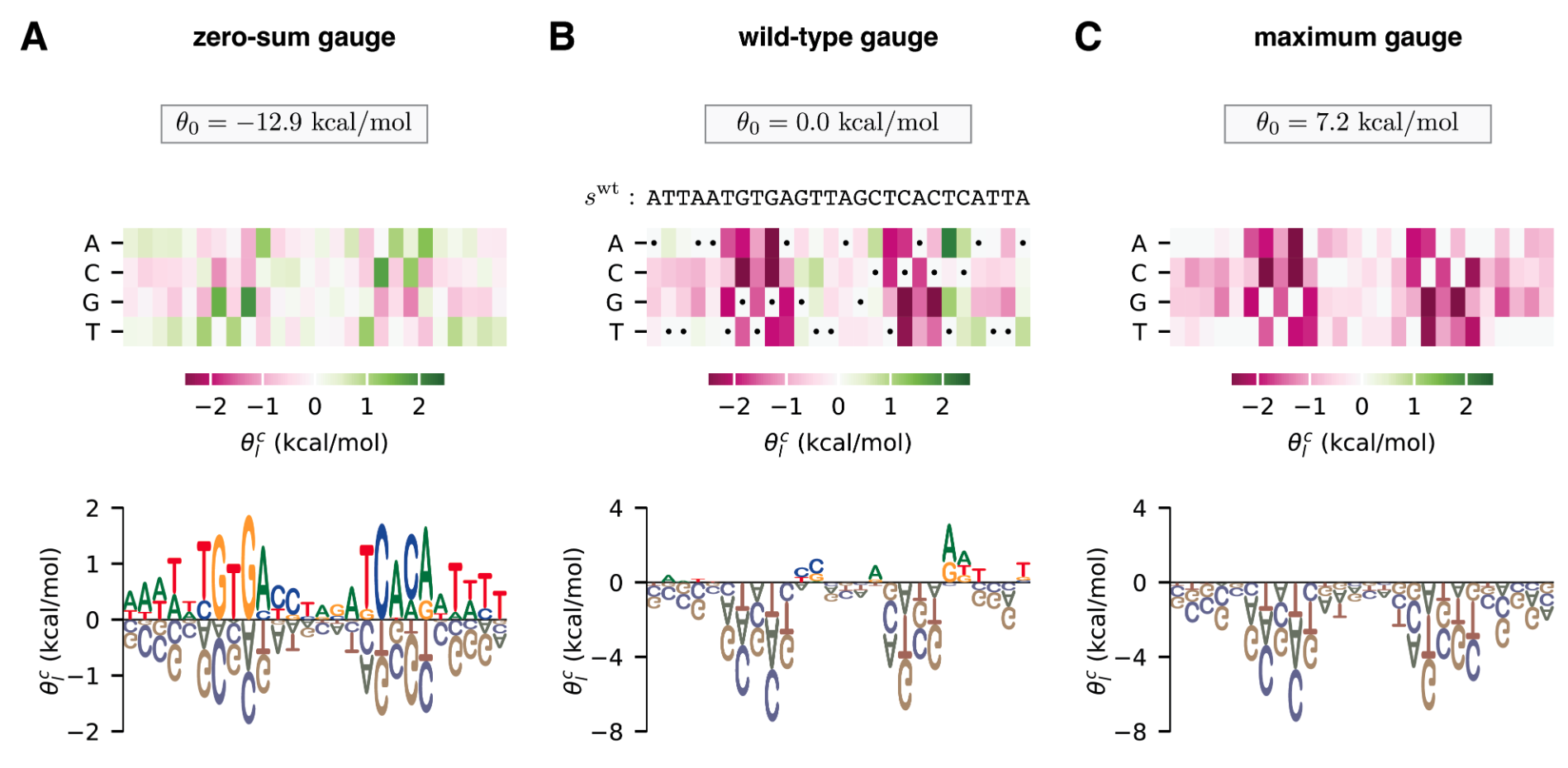Can see how relative to WT, most mutations are not very positive, but those that are stand out. Relative to the maximum gauge (i.e., the optimal choice at each position), every other choice is negative, but some are less negative (indicating that identity at that position is less important). The ZSG indicates certain positions that may be more important, and at each position, params all add to 0, so there’s a clean interpretation of identities that are positive vs. negative.

Gauge interpretations

ZSG: (aka Ising, hierarchical) — constant param. is the mean over all sequences, and params quantify deviations from the average. Intuitively, the params at any position must sum to 0, since they indicate above and below average. WT: (aka mismatch, lattice-gas) — constant param is WT function value and params quantify deviations from WT. In this case, the params for WT (i.e., AA identity term at each position) are 0. Maximum: constant param is the maximum function value (i.e., corresponding to best sequence), and params are deviations from this. Could also imagine a minimum gauge. Seems to pose practical problems in that we may not know the true maximum, though choosing observed maximum may be equivalent to a WT gauge choice. Here, at every position, at least one param is 0. Notably, this gauge is nonlinear.

Gauge spaces

Any parameter vector \(\theta\) has a corresponding “gauge orbit” \(\mathcal{O}(\theta)\equiv \{\theta + g\; : \; g \in \mathcal{G}\}\). When we fix a gauge, we restrict \(\theta\) to be in \(\Theta\) (a “gauge space”) that intersects \(\mathcal{O}(\theta)\) at exactly one point, for each \(\theta \in \mathbb{R}^M\). This yields a gauge-fixed value of \(\theta\), \(\theta_{\text{fixed}}\). There are generally an infinite number of possible choices of gauge space \(\Theta\).

Linear gauges

Def. linear subspace of the feature space. For a linear gauge \(\Theta\), \(\exists \; P \in \mathbb{R}^{M\times M} \; : \; \theta_{\text{fixed}} = P \cdot \theta_{\text{initial}}\). In words, there exists a projection matrix \(P\) that will project any vector in \(\Theta\) to an equivalent (def. by model predictions being the same) vector also in \(\Theta\). Note that \(P\) is only an orthogonal projection for \(\Theta = \matcal{S}\)⁴ Benefit: tractable. Will focus on for rest of paper. Important property: for any \(\theta_{1}, \theta_{2}\in \Theta\), \(\theta_2-\theta_1\in\Theta\) as well. This enables model comparison within the same gauge (??).

Constrained optimization view

Can also gauge-fix via constrained optimization. Specify a penalization matrix \(\Lambda\) for which there is a corresponding projection matrix as well: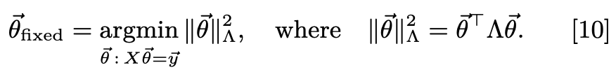 This implies that inference w/ a PD \(L_2\) regularizer on the model parameters will result in gauge-fixed params. However, regularization also changes the model predictions, so this isn’t proper. Regularization can also be specified at model prediction time, but this still requires specifying a linear gauge choice.

Unified approach to gauge fixing (p 4-6)

Focus on fixing gauge of all-order interaction model. Then, discussion of hierarchical gauges which can be applied to commonly-used models that are not all-order. 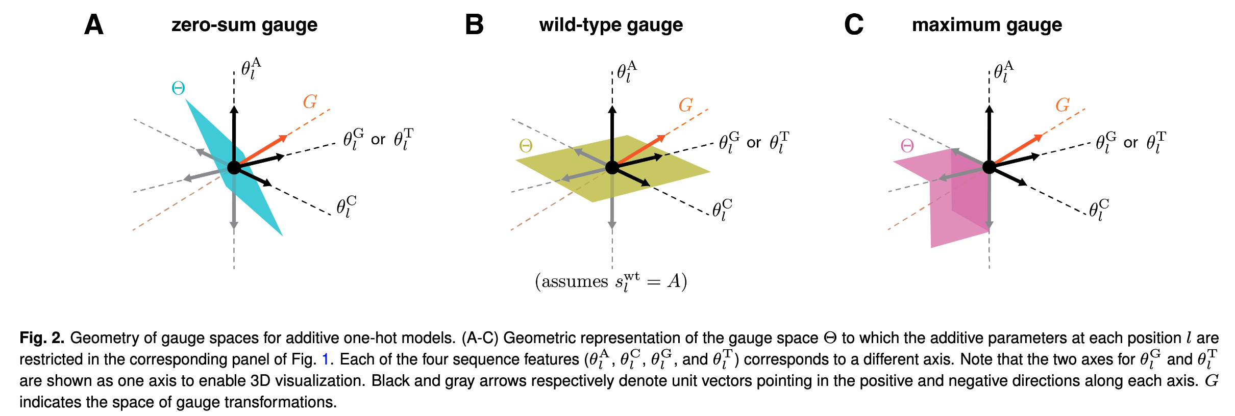Figure shows the gauge space as colored plane, where you can move the black dot around and keep predictions the same. Notably, in WTG moving around the plane involves the param for \(A\) (WT) staying fixed at 0. In MG, the black point is already the maximum so all params must be negative w.r.t. it. The ZSG demonstrates how to increase along the \(A\) param dimension, a decrease along \(G\) or some other dimension must be incurred, such that the params continue to sum to 0.

All-order interaction models

Wild-card formulation

We can express an all-order interaction model via regex: add wild-card * to the alphabet, let feature set be all possible regex s.t. \(x_{s'}(s) = 1\) if \(s\) matches pattern \(s'\) and 0 otherwise. Then clearly we can write \(f\) as a weighted (by params) sum of features \(s' \in \mathcal{S}\). A more straightforward way of writing this model is shown in Eq. 4 as a weighted sum over all interaction terms. Here the wildcard symbol encapsulates the idea of an interaction term (in that the other positions can be anything) in a slightly different framing that is a little more compact. Note also that we can factorize \(x_{s'}\) over positions by thinking of the positions in a one-hot manner. In particular, \(x_{s'}(s) = \prod_{l=1}^{L} x_l^{s_l'}(s)\) where each factor is 1 only if \(s\) has identity \(s_l'\) at position \(l\) (with wildcard always being 1). We can also write the full embedding then as a tensor product (??) over positions \(l\), where each position is represented by embedding vector where each element corresponds to one alphabet identity. What I think this means is you get an L-dimensional tensor which is flattened into a vector of size (alphabet + 1)\(^L\).

Parametric family of gauges

Define two parameters, \(\lambda \in \mathbb{R}_+\) (how much higher vs. lower order sequence features are penalized⁵) and \(p \in \Delta^{20^L}\) (probability distribution on sequence space governing how strongly the AAs @ each position are penalized) assumed to be of the form \(p(s) = \prod_{l=1}^{L} p_l^{s_l}\). We can write out the gauge space and the full parametric gauge as a tensor product, but this is a bit beyond me atm. This includes an explicit formula for \(P\), and we can also define \(\Lambda\) similarly. \(\lambda\) is involved in \(\Lambda\) raised to the order power (\(\lambda^{o(s')}\)) which is how it concretely modulates penalties depending on order; \(\lambda = 1\) yields equal weighting, \(\lambda \lt 1\) yields more penalty on lower-order terms, and \(\lambda \gt 1\) more penalty on higher-order terms. \(p(s)\) provides a weight in the usual (scalar) way.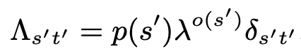

Trivial gauge

Choose \(\lambda = 0\). Then all params of order \(\lt L\) are 0, and the function value is just the full-order parameter for each sequence. \(p\) plays no role. This is effectively a look up table.

Euclidean gauge

Choose \(\lambda=\alpha\) (the size of alphabet), \(p\) the uniform distribution. This makes the penalizing norm simply the standard \(L_2\) norm. Still don’t understand comments about orthogonality. Corresponds to \(L_2\) regularization where \(\Lambda\) is a positive multiple of identity. What degrees of freedom is this removing? How to think about?

Equitable gauge

Choose \(\lambda=1\), let \(p\) vary. This gauge penalizes parameters relative to how many times they’re used, i.e., in the space of landscape contributions instead of directly in parameter space.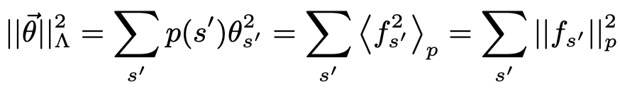

Hierarchical gauge

\(\lambda \rightarrow \infty\), let \(p\) vary. In this gauge, params obey the marginalization property: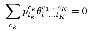

Implications of marginalization property

1) The mean activity over sequences matched by regex \(s'\) can be expressed as a simple sum of params. See examples for more detail. This means that the params can be expressed as differences of average values. Can interpret params as average mutational effect, given sequences are drawn from \(p\), beyond lower-order epistatic effects. This gauge corresponds to ANOVA decomposition. 2) The landscape naturally decomposes into mutually orthogonal components (??). This implies that the variance of the landscape w.r.t. \(p\) is the sum of contributions from interactions of different orders. This also implies that this gauge minimizes variance attribution in a hierarchical matter, prioritizing higher-order terms, and within orders, penalizing in proportion to fraction of sequences a param applies to⁶. 3) Preserves form of OHE models (equivalent to all-order interaction models, fixing certain params to 0), “hierarchical models”, including all-up-to-order-\(r\) models and nearest-neighbor interaction models (??). Guaranteed to give params where “appropriate entries” fixed to 0 still.

Zero-sum gauge (ZSG)

\(p\) is the uniform distribution. When \(p\) is uniform, Eq. 24 (shown @ Hierarchical-gauge) simply becomes the sum of params (equaling 0). Does this gauge have a clear interpretation, similar to WT,-generalized-WT-gauges? → I believe this can be thought of as setting \(\theta_0\) to be the average, such that all params quantify the effect of mutations relative to the average (which of course, isn’t super interpretable).

WT, generalized WT gauges

\(p\) approaches delta distribution around some WT sequence → only the params matching \(s^{\text{wt}}\) are penalized (to be zero)⁷. Then the various params quantify the effect of mutations of various degrees to the WT. The generalization is allowing \(p\) to put mass on multiple alleles at each position, with the stipulation being that some alleles are still set to 0 mass.

Applications (p 6-?)

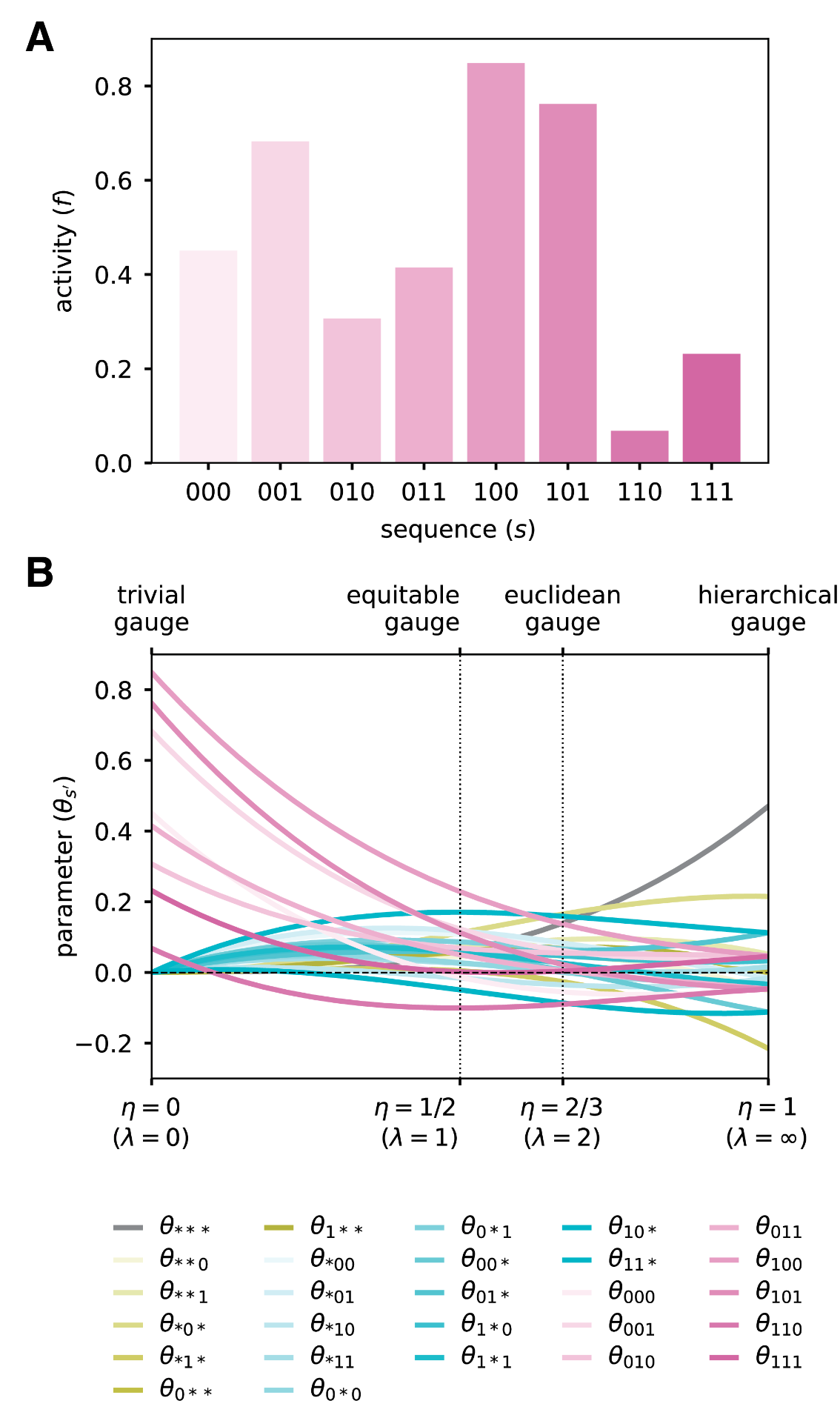\(p\) is uniform distribution, plot in B varies \(\lambda\). Hierarchical gauge corresponds to ZSG here, notice symmetry about 0. Also notice that the lower orders have more spread about zero, and higher orders have less spread about 0. Euclidean gauge has all orders distributed roughly equally about 0. Equitable gauge has most spread for highest-order (pink), decreasing to lowest order. Trivial gauge of course sets everything except the highest order terms to 0, and these are set to their function values.

Fig. 5 is also cool proof of concept: converting into linear additive model in certain localities captures almost all of the variance in that locality. While uniformly sampled sequences w/ uniform additive model have \(R^2=.59\), the region-specific ones have close to 1 on sequences from that region.

Connections

Companion paper: Symmetry, gauge freedoms, and the interpretability of sequence-function relationships | bioRxiv

Relevance

See Walsh-Hadamard Transform. WHT generally use a WT-reference gauge by default, but there hasn’t been much discussion / awareness of gauges in this literature so far.

Footnotes

1. Note that \(g\) is in the same space as \(\theta\). ↩

2. Because \(g\) provides a set of coefficients such that the columns add to 0, implying that one of the columns can be rewritten as a linear combination of the other columns. ↩

3. \(c\) is AA identity; we know that for a given position only one AA can be active; so sum is 1. ↩

4. I still don’t get what this means or why it matters. ↩

5. Seems in similar spirit to Renzo epistatic regularization schematic. Should follow up on. And is there an easy way to extend this to specify strengths on each order as percentages or something? ↩

6. This is important statement, want to understand why / its derivation. ↩

7. Excepting \(\theta_0\), which is exactly the function value of \(s^{\text{wt}}\). ↩